Interpolation search revisited
| Author: | Wojciech Muła |
|---|---|
| Added on: | 2014-09-25 |
Contents
Introduction
Interpolation search is the modification of binary search, where the index of a "middle" key is obtained from linear interpolation of values at start & end of a processed range:
a := start
b := end
key := searched key

while a <= b loop
    t := (key - array[a])/(array[b] - array[a])
    c := a + floor(t * (b - a))

    -- in binary search just: c := (a + b)/2

    if key = array[c] then
        return c
    else if key < array[c] then
        b := c - 1
    else
        a := c + 1
    endif

end loop
The clear advantage over basic binary search is complexity O(loglogn). When size of array is 1 million, then average number of comparison in binary search is log2n = 20. For interpolation search it's log2log2n = 4.3 — 4.5 times faster.
However, this property is hold only when the distribution of keys is uniform. I guess this the reason why the algorithm is not well known — enforcing uniform distribution on real data is hard. Also calculating the index c is more computational expansive.
Experiment
In the experiment array of integers was filled with ascending numbers scaled by function indexexponent, modelling different distributions. Size of array was 10'000 or 100'000 elements and exponent vary from 0.1 to 100.
Then every key in range 0 .. array size was searched using both binary and interpolation algorithm. Two values were measured:
- clock time to complete whole search;
- average number of calculating a "middle" index.
Test programs were run on quite old Pentium M, floating point calculations were done on FPU (I've tried also SSE, but improvement was minimal or none).
Results
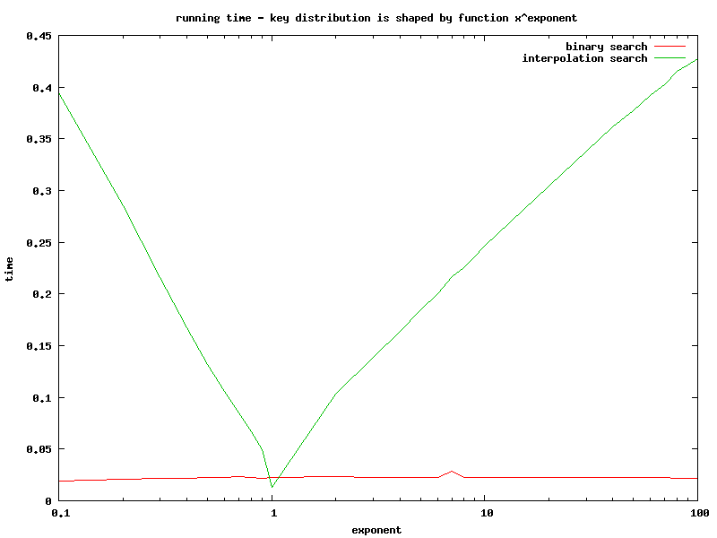
Clock time in function of exponent value.
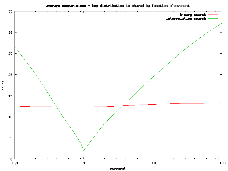
Average comparisons in function of exponent value.
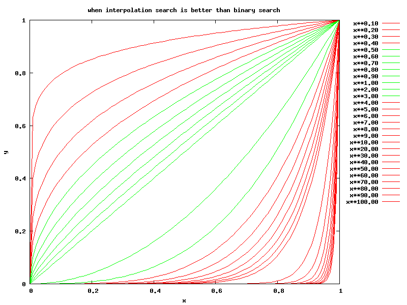
Functions xexponent — green curves are distributions for which interpolation search is better than binary search.
Summary
- The experiment proved the main property of interpolation search.
- However computational complexity of interpolation search is very sensitive to the key distribution. In the worst case it's 8 times slower and average number of comparisons is 2,5 times larger than binary search.
- Binary search keeps constant running time & number of comparisons.
Conclusion: keep away from interpolation search unless you can prove that your data has uniform distribution.
Source code
Sample programs are available at github.